|
Quantified Programs applied to Runway Scheduling
The following QIP problem definition and, as a
consequence the content of this page, is a result of
cooperative work between University Siegen (S. Gnad,
M. Hartisch, U. Lorenz) and FAU Erlangen (L. Hupp,
F. Liers, A. Peter). We used QIPs to model and solve
a matching problem that can be interpreted as an
airplane scheduling problem in which each airplane must
be assigned to a time slot and at most b airplanes can
be assigned to one time slot. This b-matching is
enhanced by uncertain time intervals in which an
airplane must land. For reasons of simplicity we will
use the airplane scheduling interpretation to explain
our intentions.
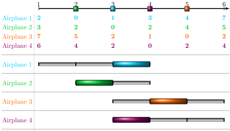
Figure 1: Example with 4 airplanes and 6 possible time
slots. 2 airplanes can be scheduled at each time slot
(b=2). The initial planning costs are given and the
possible time windows (consisting of two time slots)
for each airplane are depicted as sliders below.
Broadly speaking, we are interested in an initial plan
that can be fixed cheaply if the mandatory time windows
(the sliders in the figure) for some planes do not
contain the initially scheduled time slot. Reasons for
such variations (in the arrival time) might be adjusted
airspeed (due to weather) or operational problems.
The incurred costs are composed of the costs for the
initial plan and the fixing costs. The costs for the
initial plan only depend on the the initial assignment
of planes to time slots regarding predetermined costs:
In the example above assigning airplane 2 to time slot
4 would result in costs of 2 monetary units.
There are some ideas for the composition of the fixing
costs, for example:
-
rescheduling one airplane results in a fixed fee
-
rescheduling one airplane results in costs depending
on the newly selected time slot
-
rescheduling one airplane results in costs depending
on the initial and the newly selected time slot
For simplicity and a more general presentation, the
costs of replacing airplane i depend on a function
f(x_i*,y_i*) representing the relation between initial
plan, fixed plan and fixing costs. Depending on the
selected cost type, this function can be modeled using
linear constraints.
Basic quantified program for the airplane runway
scheduling problem:
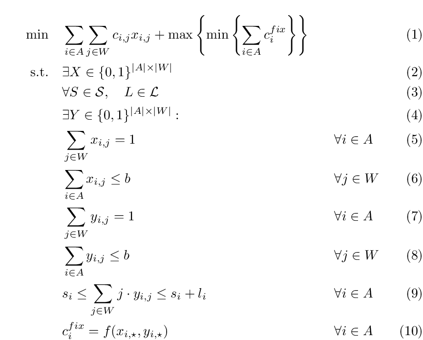
Brief explanation of the model:
-
three stage objective function
-
first stage: select initial plan resulting in
initial costs
-
second stage: uncertain events → new conditions
regarding allowed time slots (the start
(si∈S) and the length (li
∈L) of the time window is selected for each
airplane i)
-
third stage: if necessary fix the initial plan
causing additional costs
-
First stage existential variables: Initial
scheduling variables
-
Second stage universal variables: Specification of
the starting point (s) and the length (l) of the
mandatory time window for each airplane
-
Third stage existential variables: Final scheduling
variables respecting the time windows defined in
stage two
-
Ensures that each airplane is assigned to exactly
one time slot in the initial plan
-
Ensures that each time slot can only hold b airplanes
in the initial plan
-
Ensures that each airplane is assigned to exactly
one time slot in the fixed plan
-
Ensures that each time slot can only hold b
airplanes in the fixed plan
-
Binds the assigned time slots of the fixed plan to
the given time window
-
Fixing costs depend on difference between initial
plan (X) and fixed plan (Y); various cost models
imaginable.
|
|
Example costs: fixed fee
If, for example, the first mentioned fixing costs were
used, i.e. fixed fee for replanning, further existential
variables Z∈{0,1}|A|×|W| are installed in
the third stage and the following constraints would be
added:

In this case variable zij must identify if
airplane i was not scheduled in time slot j in the
initial plan but in the fixed plan resulting in costs
f for this plane.
|
|
Restricting the universal variables
By choosing the domains of the universal variables S and
L carefully the user already can limit the influence of
the universal variables. Nevertheless, some scenarios
should not be considered: For example one might want to
allow the time windows for some airplane to consist of
only one time slot. However, this should not be the case
for all airplanes, since this would constitute a rather
implausible event. One conceivable demand for the time
windows could be that on average the time windows have a
length of 2 (i.e. consist of two time slots). Thus, the
universal variables L should not only be forced to lie
within some bounds, but also within a specific polytope.
The polytope for this example would require the
following additional constraint:

However, simply adding this constraint to the constraint
system would not have the desired effect. In fact, it
would increase the influence of the universal variables
since this constraint could easily be violated and thus
the entire instance would become infeasible. However,
adding this as a universal constraint would do the trick.
or the enforcement of rules regarding the universal
variables could be performed implicitly: In a final
existential block the fulfillment of such a constraint
is checked and if a violation is detected the remaining
constraint system is relaxed and the objective value is
reduced dramatically. This has the effect that a
violation provoked by the allocation of universal
variables results in a very good objective value
(regarding the existential objective of minimization)
and is thus unfavorable with respect to the universal
maximization objective.
|
|
Instances
For this runway scheduling problem we created several
instances with several variations:
-
Instances with more than 3 stages: After the initial
plan the time windows for some
airplanes are selected by the universal variables.
For these airplanes a fixed plan must be prepared.
After that the time windows for the remaining
airplanes are specified by the universal variables
and once again the plan must be fixed.
-
Instances with restricted universal variables:
As explained above, the universal variables
determining the interval lengths must obey some rules.
-
Instances with different objective function: the
first (fixed fee) and third (distance from initial
and final time slot) presented fixing costs are
considered.
-
Instances with diverse time windows: The interval
length can vary from 0 up to 4 time slots and the
interval itself can start at up to 4 time slots.
-
Instances with different numbers of airplanes and
time slots: the number of airplanes varies between 5
and up to more than 100. The number of time slots
varies between 7 and up to 200 time slots.
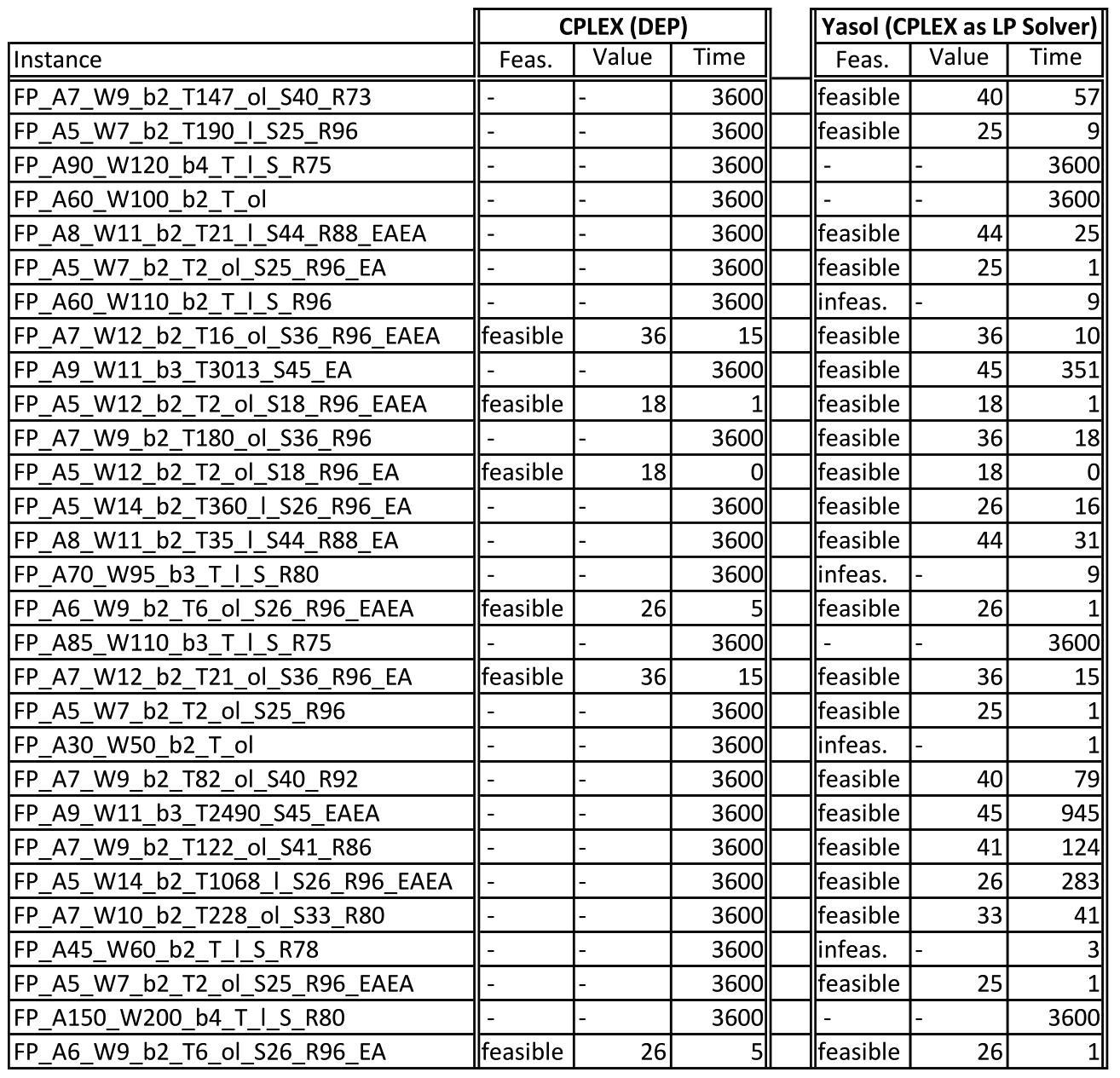
Download Instances
For each of these 29 instances our solver Yasol
(utilizing the Cplex LP solver) had one hour to solve
the instance. The results where compared to Cplex
trying to solve the corresponding deterministic
equivalent program, also within one hour. The results
are displayed in the following table. Yasol solves 25
out of the 29 instances while CPLEX only can solve 6
of the converted DEPs. Even when only considering the
instances solved by CPLEX, Yasol only needs 2.66 seconds
on average compared to 6.83 seconds. If instances get
large (easy indicator is the number right after the 'A'
in the instance name) Yasol is able to detect infeasible
instances rather fast but does not manage to grasp
optimal feasible solutions. CPLEX, on the other hand,
often exceeds the available memory on such instances
and does not cope very well if many universal variables
are present. But even on instances with few universal
variables CPLEX quickly reaches its limit.
[1] Hartisch M., Ederer T., Lorenz U., Wolf J. (2016)
Quantified Integer Programs with Polyhedral
Uncertainty Set. In: Plaat A., Kosters W., van den
Herik J. (eds) Computers and Games. CG 2016. Lecture
Notes in Computer Science, vol 10068. Springer, Cham
|
|
Downloads
Yasol for Mac OS
Yasol for Linux
Yasol for Windows
Instances
|